This is the sixth live-blog of my spring 2026 DERs class.
The last few posts discussed what Distributed Energy Resources (DERs) are and why someone might want to learn about them. This post marks a shift from the first, introductory section of the class — on definitions, motivations, and context (social, political, economic) — to the second, more technical section on DER modeling and simulation.
Mathematical modeling helps us understand how DERs work, how to design and size DER systems, and how to operate DERs to reduce energy costs, pollution, and strain on electrical infrastructure. Simulation just means running a mathematical model on a computer.
For any given DER, detailed modeling that captures all of its subtle physical effects is hard. Fortunately, one simple modeling approach captures the dominant physics of almost all of the DERs we’ll study this semester: Batteries, electric vehicles, space heating and cooling systems, water heaters, and thermal storage. That simple, broadly applicable approach is to model DER dynamics using first-order linear ordinary differential equations.
“First-order linear ordinary differential equations” is a mouthful. The lectures define each of those words precisely, with examples. To avoid getting bogged down in math, this post will just introduce the canonical DER example — a battery — which (perhaps surprisingly) ends up being almost all we need.
We’re all familiar with batteries from our personal electronics. Batteries take in electrical energy, convert it to chemical energy, store it, and convert it back to electrical energy later.
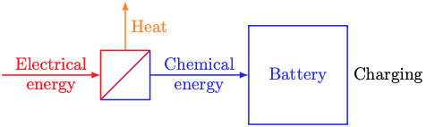
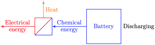
As shown above, converting between electrical and chemical energy always entails some heat loss to the battery’s surroundings. You can feel the heat if you touch your phone or laptop while it’s charging.
Next week, we’ll learn a bit about electrochemistry and model energy conversion losses. For now, we’ll just model the chemical energy dynamics (the blue stuff in the sketches above). The simplest model of a battery’s chemical energy dynamics is
Rate of change of stored energy = Charging power.
When the righthand side is positive, the battery is charging and the stored energy increases. When the righthand side is negative, the battery is discharging and the stored energy decreases.
This is about the simplest imaginable example of a first-order linear ordinary differential equation. The variable is the stored energy, a function of time. The equation is differential because it involves the derivative (rate of change) of the stored energy. It’s ordinary because the stored energy is a function of one scalar variable (time), rather than multiple variables. It’s first-order because the first derivative is the highest derivative in the equation. It’s linear because it doesn’t involve any nonlinear functions (powers, roots, sinusoids, exponentials, etc.) of the stored energy or its derivatives.
Given an initial stored energy E(0) and the charging power p(t) at each time t > 0, solving the differential equation (or more precisely, the initial value problem) means finding a function E that takes any t > 0 and returns the stored energy E(t). In this very simple example, the solution is
E(t) = E(0) + Integral of p from 0 to t.
(This formula comes from integrating both sides of dE(t)/dt = p(t) and applying the fundamental theorem of calculus.) If p is constant, then E(t) = E(0) + pt, which looks like constant-velocity motion from high school physics.
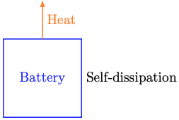
This model does not quite satisfy conservation of energy. To see why, suppose the charging power is zero: No charging, no deliberate discharging. In this case, the model predicts E(t) = E(0) for all t. Constant stored energy, forever. This contradicts our physical experience. If I fully charge a AA battery, then toss it in a junk drawer and forget about it for a year, will it still be fully charged? No, it will be dead. This means the model is missing an energy flow.
The missing energy flow is called self-dissipation: The slow, passive loss of stored chemical energy as heat dissipation to the battery’s surroundings. Self-dissipation happens even when the battery is not being actively charged or discharged.
It turns out that self-dissipation happens faster if the battery is closer to fully charged. You can convince yourself of this through a simple (if very slow) experiment. Fully charge an old electronic device, then unplug it and turn it off. Every day around the same time, turn it on, record its state of charge, and turn it off again. I bet you’ll find that the energy lost from one day to the next gets smaller as the days go by.
This observation motivates modeling self-dissipation as
Self-dissipation = Stored energy / Time constant.
The time constant, in units of hours, tells us how long it takes to lose a given amount of energy. Batteries with longer time constants have slower self-dissipation. After three time constants, the battery loses about 95% of its initial stored energy. Lithium-ion batteries — the dominant battery technology for almost all applications today — typically have time constants on the order of a thousand hours.
Adding self-dissipation to our battery model gives
Rate of change of stored energy = Charging power – Stored energy / Time constant.
Now the variable (the stored energy) shows up both directly on the righthand side and indirectly on the lefthand side via its derivative. The equation is still differential, ordinary, first-order, and linear. Some math shows that if the charging power p is constant, then the solution E(t) is a mixture of the initial state E(0) and a final value E(∞) that the stored energy asymptotically approaches but never reaches. The final value is the product of the charging power and the time constant. As time goes on1, the mixture contains more of E(∞) and less of E(0).
The battery model is canonical: It tells us almost everything we need to know about the essential dynamics of batteries, electric vehicles, space heating and cooling systems, water heaters, thermal storage, and other DERs. The battery model is so broadly applicable because it captures the essential behavior of energy storage. Although it might not be obvious now, we will see that all of the DERs mentioned above store some form of energy. Modeling these DERs using first-order linear ordinary differential equations will make the analogy to batteries clear.
The battery model is scalar: It summarizes the state of the battery by a single number. Sometimes, one number is not enough to summarize the state of a DER system. We’ll model those cases using vector first-order linear ordinary differential equations. These work about like the scalar version, but are much more powerful because they can model arbitrarily large, interconnected systems. The enabling math is called linear algebra. We’ll spend some time on it because it’s useful for DERs, but also for an incredibly wide range of computational applications that spans almost every technical field.
- More specifically, in the weighted average at time t, the weight on E(0) is the exponential of -t divided by the time constant. The weight on E(∞) is one minus the weight on E(0).